|
|
Post by antigua on Jan 13, 2017 22:54:22 GMT -5
In all of my homemade guitars instead of a regular tone control I implemented what I call 'fatness' control, which is all passive. My passive circuit uses a large-value inductor of 1H (that is not a typo) in conjunction with a capacitor and forms a tank circuit to scoop out the mids to a variable extent depending on the rotation of the knob. I simulated it using old-fashioned SPICE many years ago. It allows the guitar tone to be 'thinned' but still preserve the clarity of the attack, and as a result it totally changes the character of the pickup (makes the bridge pick become more 'gentle' than the neck pickup when set to the lowest 'fatness' level). I have never yet used it on the bridge pickup - since those large-value inductors were expensive components - but I might try swapping the bridge and neck tone controls sometime to see how it sounds. Mixing pickups with this control in place adds another dimension to the variety of tone settings it can achieve, and I am still discovering new ways to set it that I never tried before. I was never comfortable with using batteries in my guitars, so my goal was to arrive at a passive tone control solution that would have a stronger effect than conventional controls do. IMHO my design achieved that. That sounds a bit like a traditional Veritone with a fixed cap value. I had no idea what a Veritone really did until I modeled it with LTSpice and saw that it notched out mids at various frequencies. I think something like that could bring a lot of versatility to single pickup guitars, like the Fender Esquire. |
|
|
|
Post by Charlie Honkmeister on Jan 14, 2017 2:44:02 GMT -5
BTW all of the wiring mods/switching arrangements we have all tried over the years should still be valid with this approach but I prefer to use volume controls after the buffer and, I have no (or vary little) use for passive tone controls as a pot, any more after doing this and hearing the results. -Charlie In all of my homemade guitars instead of a regular tone control I implemented what I call 'fatness' control, which is all passive. My passive circuit uses a large-value inductor of 1H (that is not a typo) in conjunction with a capacitor and forms a tank circuit to scoop out the mids to a variable extent depending on the rotation of the knob. I simulated it using old-fashioned SPICE many years ago. It allows the guitar tone to be 'thinned' but still preserve the clarity of the attack, and as a result it totally changes the character of the pickup (makes the bridge pick become more 'gentle' than the neck pickup when set to the lowest 'fatness' level). I have never yet used it on the bridge pickup - since those large-value inductors were expensive components - but I might try swapping the bridge and neck tone controls sometime to see how it sounds. Mixing pickups with this control in place adds another dimension to the variety of tone settings it can achieve, and I am still discovering new ways to set it that I never tried before. I was never comfortable with using batteries in my guitars, so my goal was to arrive at a passive tone control solution that would have a stronger effect than conventional controls do. IMHO my design achieved that. Ever since I bought the Torres passive midrange control a number of years (>10) ago, and discovered that it used (as well as RC networks and a pot) an inexpensive miniature transformer to provide about a 1 H (I think) inductor, I've been fascinated with using passives to modify tone as well. Not everyone understands how nicely a passive midrange, or a Bill Lawrence Q-Filter, can help you re-voice the instrument and allow you to get beautiful clean, almost acoustic at times, sound. What worked best for me pickup-wise, was to get a hot (say, 10-15K ohms DCR) but not too hot (>15K DCR ) pickup to work with the passive midrange/LCR/Q-filter. I'm definitely digging my current active approach but most of the great recorded guitar sounds were made with passive instruments. I'm sure I and a lot of other players will always have one or more in the corral. Just agreeing from experience with what Antigua has been saying here in the thread, If you have a good LCR meter (Extech or DE-5000 or better), and an EDA tool like LTSpice or Circuitlab, you can very easily (albeit a bit draggy at times,) nail down component values with simulation to make a passive solution work well. You can save umpteen times the hours over the strategy of just messing with things until they sound good. Again, many, many thanks to Antigua for taking the time to actually do an illustrated LTSpice tutorial. (I'm so proud of myself. I steered back on topic.  ) |
|
|
|
Post by antigua on Mar 12, 2018 3:12:10 GMT -5
Something random I just came across: ieeexplore.ieee.org/document/1015185/?reload=true It still blows my mind that eddy currents somehow act as a parallel resistance as opposed to a series resistance, but here is another source talking about modeling them as such. OTOH, we see eddy current "shunting" increase with frequency, where as real shunt resistance is not frequency dependent. |
|
|
|
Post by blademaster2 on Mar 28, 2018 15:25:53 GMT -5
Antigua- I assume you mean "capacitor", not "resistor". Since this is a step-by-step tutorial for the uninitiated, typos should probably be corrected for clarity.  But, yes, great work! I won't move this thread, as it does relate to pickups certainly, but I think you should probably repost this in the "References" section as well. On the topic of capacitors: Antigua, your SPICE circuit seems to be achieving a close result to lab measurements so I would say your model is pretty accurate. I see, however, that the Tone control resistance is tied straight to ground whereas in typical tone control circuits I see (different from my own guitars) it would have a capacitor between the Pot resistance and ground. I gather it makes little difference since you are already so close. In my admittedly-weird guitar circuits I *do* tie the pot to ground, but I have tested it with this ground connection opened up and hear no difference at all. |
|
|
|
Post by newey on Mar 28, 2018 16:57:25 GMT -5
The model is based upon the assumption that the tone control is at "10", and there the capacitor is effectively out of the circuit. It can therefore be ignored for purposes of the model.
|
|
|
|
Post by antigua on Mar 29, 2018 21:05:22 GMT -5
Antigua- I assume you mean "capacitor", not "resistor". Since this is a step-by-step tutorial for the uninitiated, typos should probably be corrected for clarity. But, yes, great work! I won't move this thread, as it does relate to pickups certainly, but I think you should probably repost this in the "References" section as well. On the topic of capacitors: Antigua, your SPICE circuit seems to be achieving a close result to lab measurements so I would say your model is pretty accurate. I see, however, that the Tone control resistance is tied straight to ground whereas in typical tone control circuits I see (different from my own guitars) it would have a capacitor between the Pot resistance and ground. I gather it makes little difference since you are already so close. In my admittedly-weird guitar circuits I *do* tie the pot to ground, but I have tested it with this ground connection opened up and hear no difference at all. That's a good question. I don't recall the circumstances around that decision, I think the assumption was that the cap didn't matter with a large resistance in series with it. I just made a pickup model with the cap in series with the resistor, and it does change the impedence slightly:  The larger cap value decreased the resonant amplitude by 1dB to 2dB, and raised the resonant frequency by a tiny amount. That would be hard to hear, in fact I have several guitars with cap selectors built in, and I could never tell the difference when the tone knob was at 10. |
|
|
|
Post by JohnH on Mar 29, 2018 22:54:48 GMT -5
I was probably in that discussion about the tone cap earlier on. I think that for lab testing its definitely the right thing to keep a consistent simple extra load for the loaded tests, cap and resistor but not with tone cap. The tone cap doesnt make much difference at full tone, as you show above. And some guitars have none anyway, such as bridge pickups on Strats which either have no tone pot or a no-load one.
|
|
|
|
Post by antigua on Mar 30, 2018 1:29:51 GMT -5
The dummy load for "loaded" tests is just one cap and one resistor, but I favor that arrangement on account of the fact that it's simple, approximate and consistent. For modelling, I think because there was a 1 to 2dB difference at resonance, it's worth adding to the model. I found something interesting:  If I understood circuit analysis better then the reason would probably be apparent, but the resonant peak drops abruptly, from the high point to the low point, as the capacitance value increases from 25pF to 100pF. In the screen shot above, the dark green line, dark blue and beige in the middle of the cluster are 50pF , 75pF and 100pf, for reference. Once it gets to about 150pF, higher capacitance values have no further effect on the minimum amplitude, while values at or below 1pF make no difference to the maximum amplitude. If the 500p cable and the 120p pickup values are changed, this threshold changes, but for different pickup inductance and resistance values, it stays nearly the same, meaning it's mostly, maybe entirely, interactive with the parallel capacitance. tl;dr, for a given overall parallel capacitance, there will be a particular tone cap value range across which it transitions from a maximum to a minimum effect. Given that a typical 22nF or 47nF cap have large values compared to the pickup and cable, they will produce the same outcome in situ. This is probably why I never heard a difference with my guitar, I'd have to have a capacitor under 50p to realize that boost. |
|
|
|
Post by ms on Mar 30, 2018 6:25:25 GMT -5
For normal values of the tone capacitor, the magnitude of its impedance is very small compared to 500K. Example: the magnitude of the impedance of a .02 microf cap. at 4000Hz is about 2000 ohms, not significant. You can think of the tone cap. as like a coupling cap. On the other hand, the mag. of the imp. of 100pf at 4000Hz is about 400,000 ohms. This is significant and so the C has an effect, altering the loading of the tone cap even with the pot on 10. The loading of the tone pot is completely eliminated as the cap gets significantly smaller than 100pf.
|
|
|
|
Post by Yogi B on Mar 30, 2018 10:32:02 GMT -5
As for: If I understood circuit analysis better then the reason would probably be apparent, but the resonant peak drops abruptly, from the high point to the low point, as the capacitance value increases from 25pF to 100pF. As ms describes the smaller the cap the larger the impedance (well it's magnitude, it's negative imaginary part, or negative reactance). At small cap values the tone circuit appears like an open circuit, at least for the frequencies we're concerned with -- for larger values it appears closer to a short, therefore the tone control is essentially just the 500kΩ resistance of the pot. Thus the output range of the varied capacitance is between the limits of no additional loading to 500kΩ of it. Since the difference between the no-load and 500kΩ responses is concentrated to the resonant peak, the value of the cap is going to have most effect when the cutoff frequency of the filter formed is in the same range, with little effect when either side of it. |
|
|
|
Post by antigua on Mar 30, 2018 10:48:43 GMT -5
For normal values of the tone capacitor, the magnitude of its impedance is very small compared to 500K. Example: the magnitude of the impedance of a .02 microf cap. at 4000Hz is about 2000 ohms, not significant. You can think of the tone cap. as like a coupling cap. On the other hand, the mag. of the imp. of 100pf at 4000Hz is about 400,000 ohms. This is significant and so the C has an effect, altering the loading of the tone cap even with the pot on 10. The loading of the tone pot is completely eliminated as the cap gets significantly smaller than 100pf. Thanks, that makes perfect sense. So having no cap at all is essentially the same as having a a high value cap, but a low value cap cuts off that route, therefor decreasing the load on the pickup. Here is a model showing a 47nF cap in circuit, and then bypassed with low resistance, with an identical impedance curve.  |
|
|
|
Post by reTrEaD on Mar 30, 2018 18:10:45 GMT -5
Any time we start talking about impedance, it's useful to think in terms of vectors. When the capacitive reactance is very small compared to the resistance in the series combination of a shunt type treble-cut circuit, it can be convenient to ignore the effect of capacitive reactance on the cumulative impedance, both in terms of magnitude and direction. If we want to know exactly what's going on there, we need to consider the effect on both the magnitude (again, adding vectors not just simple addition) and direction. Usually considering just the resistance gets us very close to the truth.
When the ratio of resistance to capacitive reactance moves toward 1 to 1, neither the resistance or capacitive reactance alone tell us anything close to what we would want to know. At 1:1, the direction is at 45 degrees from either and the magnitude is roughly 1.4 times the resistance or capacitive reactance.
As our series circuit moves closer to a purely capacitive circuit, we can ignore the resistance, being ever mindful of the direction of the vector being at a right angle to one representing a resistance-only impedance.
When we consider the fact that the capacitive reactance of a typical 0.022µF capacitor is still below 100k at 82Hz (the fundamental frequency of the low E on a standard guitar), the effect of the resistance of the pot has a greater effect on tone during the early portion of rotation from fully clockwise than the value of the cap. It isn't terribly different than having just the pot directly connected with no cap, in that part of its range.
Things get more interesting, the farther we progress counter-clockwise. And very interesting when R=0.
|
|
|
|
Post by Yogi B on Apr 11, 2018 10:45:33 GMT -5
Any time we start talking about impedance, it's useful to think in terms of vectors. Or y'know complex numbers. Speaking of which, I find it bizarre that LTSpice doesn't have an inbuilt constant assigned to the value sqrt(-1), either i or j. Or some other nice way to specify complex numbers, say perhaps, a function that takes the real and imaginary components, or alternatively magnitude and phase. Additionally a built in NaN (not a number) constant would be nice, but that's probably only a sign I'm abusing the language in ways I shouldn't. At least it has the hyperbolic functions. |
|
|
|
Post by Yogi B on Apr 14, 2018 0:39:17 GMT -5
I've taken another stab at implementing Tillman's comb filtered responses in LTSpice using an arbitrary behavioural voltage source, taking two different approaches. The first using the delay (and idt) function(s): .param scale=25.5 f_open=110*2**(0/12) pickup_aperture=1 pickup_position=6.375
.func comb_filter(vol, delta) = {
+ (vol - delay(vol, delta)) / 2
+}
.func comb_aperture_delay(vol) = {
+ 4 * scale * f_open / pickup_aperture * idt(comb_filter(vol, pickup_aperture / 2 / scale / f_open))
+}
.func comb_position_delay(vol) = {
+ comb_filter(vol, pickup_position / scale / f_open)
+}
.func comb_delay(vol) = {
+ comb_position_delay(comb_aperture_delay(vol))
+}
V_AC ref 0 AC 1
B_delay out 0 V = comb_delay(V(ref))
The second utilising the b-source's Laplace parameter: .func comb_aperture_laplace(s, pickup_aperture, scale, f_open) = {
+ - 4 * scale * f_open / pickup_aperture / s * sinh(s * pickup_aperture / 4 / scale / f_open)
+}
.func comb_position_laplace(s, pickup_position, scale, f_open) = {
+ sqrt(-1) * sinh(s * pickup_position / 2 / scale / f_open)
+}
.func comb_laplace(s, pickup_position, pickup_aperture, scale, f_open) = {
+ comb_aperture_laplace(s, pickup_aperture, scale, f_open)
+ * comb_position_laplace(s, pickup_position, scale, f_open)
+}
V_AC ref 0 AC 1
B_Laplace out 0
+ V = V(ref)
+ Laplace = comb_laplace(s, 6.375, 1, 25.5, 110*2**(0/12))
Both give the same response in terms of magnitude, but differ in phase. Both also give much better performance than manually stepping a frequency parameter and using .AC list {freq} -- the method I had previously used. |
|
|
|
Post by JohnH on Apr 14, 2018 3:08:18 GMT -5
Don't stop there! If you want to combine Tillman's combs with the electrical modelling, then you must logically also do the bit in between, which is to model the relative amplitudes of each string harmonic (ref Jungmann). Its not too hard, I got it into excel for GuitarFreak.
|
|
|
|
Post by Yogi B on Apr 14, 2018 13:30:17 GMT -5
Don't stop there! If you want to combine Tillman's combs with the electrical modelling, then you must logically also do the bit in between, which is to model the relative amplitudes of each string harmonic (ref Jungmann). Its not too hard, I got it into excel for GuitarFreak. I assume you're essentially referring to this equation: ^2}\cdot\frac{l^2}{l_1(l-l_1)}\cdot\sin\!\left(\frac{n&space;\pi&space;l_1}{l}\right) "C_n = \frac{2h}{(n \pi)^2}\cdot\frac{l^2}{l_1(l-l_1)}\cdot\sin\!\left(\frac{n \pi l_1}{l}\right)") If so, what value are you using for h? As far as I can see there are three options: - A value dependent on fopen, l, and l1 such that the response is adjusted to be 0dB at 0Hz;
- A value dependent on fopen, l, and l1 such that the response is adjusted to be 0dB at fopen;
- Some constant independent of the other variables;
- Or, something else.
Fun Fact: In addition to the previous notes about constants in LTSpice, for some reason it appears that pi isn't defined inside Laplace expressions. |
|
|
|
Post by JohnH on Apr 14, 2018 15:12:06 GMT -5
Don't stop there! If you want to combine Tillman's combs with the electrical modelling, then you must logically also do the bit in between, which is to model the relative amplitudes of each string harmonic (ref Jungmann). Its not too hard, I got it into excel for GuitarFreak. I assume you're essentially referring to this equation: If so, what value are you using for h? As far as I can see there are three options: - A value dependent on fopen, l, and l1 such that the response is adjusted to be 0dB at 0Hz;
- A value dependent on fopen, l, and l1 such that the response is adjusted to be 0dB at fopen;
- Some constant independent of the other variables;
- Or, something else.
Fun Fact: In addition to the previous notes about constants in LTSpice, for some reason it appears that pi isn't defined inside Laplace expressions. Dead right! and the short answer is 'something else'. What I try to do is to capture as near to the real physics as is possible from the known information, based on reasonable assumptions. In the case of 'h' (which is the displacement of the string in mm), it means using a value for the string tension and the plucking force. I assume: All strings have the same tension, 7kgf = 70N. Real sets vary a bit between strings, but stay reasonably close to this and I believe a constant string tension across a set is an ideal case, suitable for analysis. Plucking is always the same force, dependent on the player and their pick From this, using the static equilibrium of a deflected string in tension, I work out the displacement. It varies according to the fretted free length of the string and how close to the bridge it is being plucked. The equation from Jungmann gives mm amplitude of the string vibration. But for the pickup output, this then needs to be scaled by frequency since pickup output is depended on rate of flux change which relates to velocity rather than displacement. Then it is turned in a db value using a 20log function, so that db differences due to this effect can be added to variations due to electrical and Tlllman comb effects to give a net result. Here is a screen shot of part the hidden GF page that works the string harmonics:  This is processing the lowest string on a 7 string guitar. This set of results is then shifted to process all other strings that are selected as active. I've posted the formulae for two key cells, being h (cell C1), and the db amplitude due to harmonics, for the fundamental (cell D19). The blue lines are indicating precedents that feed into each cell. In addition to all that, there is an arbitrary 'how hard are you plucking' constant, currently x 1.25. This is picked so that results where these effects are plotted sit nicely on graphs which also include only electrical responses. |
|
|
|
Post by JohnH on Apr 15, 2018 15:16:17 GMT -5
Just a bit more on string harmonics: If you plot out all the harmonics and their applitudes as above, they look like this:  That picture shows results from all the strings, with the blue line showing an envelope within which they all exist. This approx envelope is based on the highest active string and its simply a 6db/octave roll-off after a freqency which is about 20% higher than the fundamental. the advantage of it for plotting graphs is that it creates smooth function instead of discreet individual harmonic points. |
|
|
|
Post by Yogi B on Apr 17, 2018 13:49:59 GMT -5
pi isn't defined inside Laplace expressions. There's also issues with using Boolean related functions, most aren't defined at all and others don't seem to function correctly (max & min, even when fed with real valued numbers) -- I suppose the intention is force you to avoid discontinuities. It just means I have to roll my own: .func gt(a, b) = {floor((1 + sgn(a - b)) / 2)}
.func ge(a, b) = {ceil((1 + sgn(a - b)) / 2)}
.func lt(a, b) = {floor((1 + sgn(b - a)) / 2)}
.func le(a, b) = {ceil((1 + sgn(b - a)) / 2)}
.func eq(a, b) = {1 - floor(sgn(abs(a-b)))}
.func neq(a, b) = {floor(sgn(abs(a-b)))}
.func and(a, b) = {buf(a) * buf(b)}
.func or(a, b) = {1 - inv(a) * inv(b)}
.func if(value, on_truthy, on_falsy) = {on_truthy*buf(value) + on_falsy*inv(value)}
.func i() = {sqrt(-1)}
.func pi() = {3.14159265358979323846}
What I try to do is to capture as near to the real physics as is possible from the known information, based on reasonable assumptions. I did think about that as an option, but dismissed it primarily on the basis that I feel it's better to not have the volume level dependent the picking distance. Plus I had made that idea more complex for myself by not making sensible assumptions about what to disregard regarding the deflected string condition. Yeah, I'd already realised that when previously looking at this, I had missed that piece of the puzzle. I've ended up using a value a whole order of magnitude (and a bit) larger, at:  (≈ 13.5, for l = 25.5) which scales the response to 0dB at fopen, when picking at the midpoint of the string. Mind you I've also scaled the other comb filters too, plus I'm otherwise working in imperial -- though that should all cancel out. These are my resulting functions: .func comb_aperture(s, pickup_aperture, scale, f_open) = {
+ - 4 * scale * f_open / pickup_aperture / s * sinh(s * pickup_aperture / 4 / scale / f_open)
+ / (2 * scale * sin(pi() * pickup_aperture / 2 /scale ) / pi() / pickup_aperture) ; adjust to 0dB @ f_open
+}
.func comb_position(s, pickup_position, scale, f_open) = {
+ - i() * sinh(s * pickup_position / 2 / scale / f_open)
+ / sin(pi() * pickup_position / scale) ; adjust to 0dB @ f_open
+}
.func comb_pluck(s, pluck_position, scale, f_open) = {
+ 8 * (scale * f_open / s)^2 / pluck_position / (scale - pluck_position)
+ * i() * sinh(s / 2 / f_open * pluck_position / scale)
+ * pluck_position * (scale - pluck_position) / 70 / scale
+ * (35 * pi()^2 / scale) ; adjust to 0dB @ f_open, pluck_position = scale/2
+}
.func velocity(s, f_open) = {
+ s / 2 / pi() / i() / f_open
+}
.func response(s, pickup_position, pickup_aperture, pluck_position, scale, f_open) = {
+ 1
+ * comb_aperture(s, pickup_aperture, scale, f_open)
+ * comb_position(s, pickup_position, scale, f_open)
+ * comb_pluck(s, pluck_position, scale, f_open) * velocity(s, f_open)
; + * pluck_x_velocity_envelope(s, pluck_position, scale, f_open)
+}
This approx envelope is based on the highest active string and its simply a 6db/octave roll-off after a frequency which is about 20% higher than the fundamental. About 20%, eh? Here's what I did: .func d_pluck_x_velocity_by_ds(s, pluck_position, scale, f_open) = {
+ pi() * pluck_position * cosh(pluck_position * s / 2 / f_open / scale) / scale / s
+ - 2 * pi() * f_open * sinh(pluck_position * s / 2 / f_open / scale) / s^2
+}
.func d_reciprocal_velocity_by_ds(s, f_open) = {
+ -2 * pi() * f_open * i() / s^2
+}
.func pluck_x_velocity_envelope(s, pluck_position, scale, f_open) = {
+
+ ; Below is true if freq < freq of first null && gradient less steep than -6dB /octave
+
+ if(and(
+ lt(s / i(), 2 * pi() * scale * f_open / pluck_position),
+ lt(d_pluck_x_velocity_by_ds(s, pluck_position, scale, f_open) / i(), d_reciprocal_velocity_by_ds(s, f_open) / i())
+ ), ( ; then
+ comb_pluck(s, pluck_position, scale, f_open) * velocity(s, f_open)
+ ), ( ; else
+ 1 / velocity(s, f_open)
+ ))
+}
|
|
|
|
Post by JohnH on Apr 17, 2018 22:23:56 GMT -5
Im not good at reading code, but I'm seeing hyperbolic trig functions in there!(and I've had nothing to smoke either)
How close are you to plotting graphs with these comb and harmonic features combined with electrical effects? It would be great to compare like-with-like plots with GFreak.
|
|
|
|
Post by Yogi B on Apr 18, 2018 3:24:38 GMT -5
Im not good at reading code, but I'm seeing hyperbolic trig functions in there!(and I've had nothing to smoke either) That's from use of the identities: sin(x * i) = i * sinh(x) & cos(x * i) = cosh(x). So here's some overlayed plots of GuitarFreak's defaults (Strat Fat50 Bridge, no-load tone, etc.) but with only the 6th string plotted, full response on the left, envelope on the right. 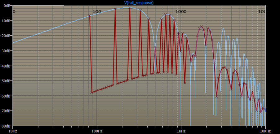 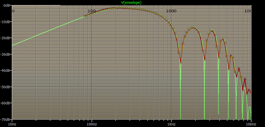 |
|
|
|
Post by JohnH on Apr 18, 2018 6:00:26 GMT -5
That looks encouraging! The differences in the high treble on the left graph are simply that only 30 harmonics per string are included in GF, so on the low E 6th string, it runs out at about 2445hz
|
|
|
|
Post by pablogilberto on Feb 26, 2020 20:16:16 GMT -5
Dynamically altering multiples component values...Often times you want to edit two or more parameters at once. Suppose you want to simulate how well a treble bleed capacitor value will retain treble as you turn down the volume knob. The problem is, a potentiometer is like two resistor value changing in tandem; the portion to the left of the wiper, and the portion to the right (voltage divider setup). The step command as shown above only provided a single value, but we need two values in order to model the two sides of the volume pot at different volume settings. The solution is an LTSpice "list" and it's "table" feature. Suppose you name your resistor variables "POT_UPPER" and "POT_LOWER" to represent the two halves of the potentiometer, and you want to plot six different points along the volume knob turn, with a different division of resistance at each point, the command would look like this: .step param COUNT list 1 2 3 4 5 6
.param POT_UPPER table( COUNT, 1,1, 2,50k, 3,100k, 4,150k, 5,200k, 6,240k )
.param POT_LOWER table( COUNT, 1,250K, 2,200k, 3,150k, 4,100k, 5,50k, 6,10k ) The first line says that you want to step through six values, using a variable called "COUNT". The second line says you want to create a table that maps all six steps of COUNT to specific values. These values will represent various resistances on one side of the pot, and assign those values to "POT_UPPER" The third line does the same thing as line two, but this time the values are inverted, in order to represent the other side of the pot, and those values are assigned to "POT_LOWER". Note that zero can't be used as a resistor value in SPICE, so "1 ohm" is used as a stand-in value. Hi antigua! Great work on this! I want to learn more about the syntax (step, param, list, table, etc.) so I can write my own codes for experimentation. Can you tell me more about this or point me to a reference tutorial? Thank you! |
|
|
|
Post by antigua on Feb 27, 2020 3:11:59 GMT -5
Dynamically altering multiples component values...Often times you want to edit two or more parameters at once. Suppose you want to simulate how well a treble bleed capacitor value will retain treble as you turn down the volume knob. The problem is, a potentiometer is like two resistor value changing in tandem; the portion to the left of the wiper, and the portion to the right (voltage divider setup). The step command as shown above only provided a single value, but we need two values in order to model the two sides of the volume pot at different volume settings. The solution is an LTSpice "list" and it's "table" feature. Suppose you name your resistor variables "POT_UPPER" and "POT_LOWER" to represent the two halves of the potentiometer, and you want to plot six different points along the volume knob turn, with a different division of resistance at each point, the command would look like this: .step param COUNT list 1 2 3 4 5 6
.param POT_UPPER table( COUNT, 1,1, 2,50k, 3,100k, 4,150k, 5,200k, 6,240k )
.param POT_LOWER table( COUNT, 1,250K, 2,200k, 3,150k, 4,100k, 5,50k, 6,10k ) The first line says that you want to step through six values, using a variable called "COUNT". The second line says you want to create a table that maps all six steps of COUNT to specific values. These values will represent various resistances on one side of the pot, and assign those values to "POT_UPPER" The third line does the same thing as line two, but this time the values are inverted, in order to represent the other side of the pot, and those values are assigned to "POT_LOWER". Note that zero can't be used as a resistor value in SPICE, so "1 ohm" is used as a stand-in value. Hi antigua! Great work on this! I want to learn more about the syntax (step, param, list, table, etc.) so I can write my own codes for experimentation. Can you tell me more about this or point me to a reference tutorial? Thank you! LTSpice is twenty years old and it's crude interface really shows it. You have to watch some YouTube tutorials to learn how to do basic things with it, or else play around with it a lot to figure out how things work. Specifically you want to know how the create a circuit, and then run the "simulate" command, so that you can see what the circuit does. The good news is that the screen shots show most of the information you need to know in order to recreate the circuits. They who the component type, the component values, the AC generator configuration, and the step table configs. Virtually nothing of importance is hidden. Here's info on how to create a multi parameter step table electronics.stackexchange.com/questions/126659/how-to-use-step-param-with-more-than-two-parameters-in-ltspiceiv/156626You might run into a lot of strange error messages as I did. If so, I can possibly help trouble shoot. Here is an asc file you can open with LTSpice for a simple pickup that uses a two parameter step table to simulate turning a volume pot down echoesofmars.com/ltspice/demo_pickup_with_step_table.asc very similar to this one:  |
|
|
|
Post by aquin43 on Feb 27, 2020 16:46:51 GMT -5
You can make pots in LTSpice as follows:
file pot.sub:

.subckt pot cw ccw s
.param newset = {(1 + (set - 1)*(set < 1)) * (set >0)}
rtop cw s {0.1+val*(1-newset)}
rbot s ccw {0.1+val*newset}
.ends pot

.subckt lpot cw ccw s
.param newset = {0.2*set*(set <= 0.5)+(1.8*set-0.8)*(set>0.5)}
rtop cw  s {0.1+val*(1-newset)}
rbot s ccw {0.1+val*newset}
.ends lpot
file pot.asy:

Version 4
SymbolType CELL
LINE Normal 16 88 16 96
LINE Normal 16 16 16 24
LINE Normal 27 24 5 24
LINE Normal 5 88 5 24
LINE Normal 5 88 27 88
LINE Normal 27 24 27 88
LINE Normal -6 39 5 48
LINE Normal -6 57 -6 39
LINE Normal 5 48 -6 57
WINDOW 0 31 40 Left 2
WINDOW 3 31 76 Left 2
SYMATTR Value val=
SYMATTR Prefix X
SYMATTR SpiceModel pot
SYMATTR Value2 set=
SYMATTR ModelFile pot.sub
PIN 16 16 NONE 0
PINATTR PinName CW
PINATTR SpiceOrder 1
PIN 16 96 NONE 0
PINATTR PinName CCW
PINATTR SpiceOrder 2
PIN 16 48 NONE 8
PINATTR PinName s
PINATTR SpiceOrder 3
file lpot.asy:

Version 4
SymbolType CELL
LINE Normal 16 88 16 96
LINE Normal 16 16 16 24
LINE Normal 27 24 5 24
LINE Normal 5 88 5 24
LINE Normal 5 88 27 88
LINE Normal 27 24 27 88
LINE Normal -6 39 5 48
LINE Normal -6 57 -6 39
LINE Normal 5 48 -6 57
TEXT 5 67 Left 2 lg
WINDOW 0 31 40 Left 2
WINDOW 3 31 76 Left 2
SYMATTR Value val=
SYMATTR Prefix X
SYMATTR SpiceModel lpot
SYMATTR Value2 set=
SYMATTR ModelFile pot.sub
PIN 16 16 NONE 0
PINATTR PinName CW
PINATTR SpiceOrder 1
PIN 16 96 NONE 0
PINATTR PinName CCW
PINATTR SpiceOrder 2
PIN 16 48 NONE 8
PINATTR PinName s
PINATTR SpiceOrder 3

Place the .sub file in LTSpice's lib/sub directory
and the two .asy files in the misc directory in lib/assy

Then, after restarting LTSpice you will have a log and a linear
pot available with parameters 'val' and 'set'
Example, showing how the pickup peak falls away as you turn down the volume:
The tset line is a comment. If it is made into a directive, both pots will vary. The log pot is a crude stepwise linear approximation. Better functions could be used, but real pots are often as crude.
Arthur
|
|
|
|
Post by pablogilberto on Feb 27, 2020 18:51:07 GMT -5
Hi antigua! Great work on this! I want to learn more about the syntax (step, param, list, table, etc.) so I can write my own codes for experimentation. Can you tell me more about this or point me to a reference tutorial? Thank you! LTSpice is twenty years old and it's crude interface really shows it. You have to watch some YouTube tutorials to learn how to do basic things with it, or else play around with it a lot to figure out how things work. Specifically you want to know how the create a circuit, and then run the "simulate" command, so that you can see what the circuit does. The good news is that the screen shots show most of the information you need to know in order to recreate the circuits. They who the component type, the component values, the AC generator configuration, and the step table configs. Virtually nothing of importance is hidden. Here's info on how to create a multi parameter step table electronics.stackexchange.com/questions/126659/how-to-use-step-param-with-more-than-two-parameters-in-ltspiceiv/156626You might run into a lot of strange error messages as I did. If so, I can possibly help trouble shoot. Here is an asc file you can open with LTSpice for a simple pickup that uses a two parameter step table to simulate turning a volume pot down echoesofmars.com/ltspice/demo_pickup_with_step_table.asc very similar to this one: Thank you for this info antiguaMuch appreciated! I will check the links and will let you know if I need any help. Cheers! |
|
|
|
Post by pablogilberto on Feb 29, 2020 19:13:05 GMT -5
You can make pots in LTSpice as follows:
file pot.sub:

.subckt pot cw ccw s
.param newset = {(1 + (set - 1)*(set < 1)) * (set >0)}
rtop cw s {0.1+val*(1-newset)}
rbot s ccw {0.1+val*newset}
.ends pot

.subckt lpot cw ccw s
.param newset = {0.2*set*(set <= 0.5)+(1.8*set-0.8)*(set>0.5)}
rtop cw  s {0.1+val*(1-newset)}
rbot s ccw {0.1+val*newset}
.ends lpot
file pot.asy:

Version 4
SymbolType CELL
LINE Normal 16 88 16 96
LINE Normal 16 16 16 24
LINE Normal 27 24 5 24
LINE Normal 5 88 5 24
LINE Normal 5 88 27 88
LINE Normal 27 24 27 88
LINE Normal -6 39 5 48
LINE Normal -6 57 -6 39
LINE Normal 5 48 -6 57
WINDOW 0 31 40 Left 2
WINDOW 3 31 76 Left 2
SYMATTR Value val=
SYMATTR Prefix X
SYMATTR SpiceModel pot
SYMATTR Value2 set=
SYMATTR ModelFile pot.sub
PIN 16 16 NONE 0
PINATTR PinName CW
PINATTR SpiceOrder 1
PIN 16 96 NONE 0
PINATTR PinName CCW
PINATTR SpiceOrder 2
PIN 16 48 NONE 8
PINATTR PinName s
PINATTR SpiceOrder 3
file lpot.asy:

Version 4
SymbolType CELL
LINE Normal 16 88 16 96
LINE Normal 16 16 16 24
LINE Normal 27 24 5 24
LINE Normal 5 88 5 24
LINE Normal 5 88 27 88
LINE Normal 27 24 27 88
LINE Normal -6 39 5 48
LINE Normal -6 57 -6 39
LINE Normal 5 48 -6 57
TEXT 5 67 Left 2 lg
WINDOW 0 31 40 Left 2
WINDOW 3 31 76 Left 2
SYMATTR Value val=
SYMATTR Prefix X
SYMATTR SpiceModel lpot
SYMATTR Value2 set=
SYMATTR ModelFile pot.sub
PIN 16 16 NONE 0
PINATTR PinName CW
PINATTR SpiceOrder 1
PIN 16 96 NONE 0
PINATTR PinName CCW
PINATTR SpiceOrder 2
PIN 16 48 NONE 8
PINATTR PinName s
PINATTR SpiceOrder 3

Place the .sub file in LTSpice's lib/sub directory
and the two .asy files in the misc directory in lib/assy

Then, after restarting LTSpice you will have a log and a linear
pot available with parameters 'val' and 'set'
Example, showing how the pickup peak falls away as you turn down the volume:
The tset line is a comment. If it is made into a directive, both pots will vary. The log pot is a crude stepwise linear approximation. Better functions could be used, but real pots are often as crude.
Arthur
I will also try this! Many thanks for the help! I hope I can learn how to code this also. Thank you! |
|
pasqualino
Rookie Solder Flinger
 Shifting gears and now "honing my axe" and building a quick Tweed F1
Posts: 10
Likes: 1
|
Post by pasqualino on Oct 18, 2020 17:08:41 GMT -5
Bra-f'n-VO! I've been using Micro-Cap which is a little more cantankerous when it comes to modeling of components. This seems to be particularly true for old transistors like our beloved AC128. I started out as an analog guy when I joined the Navy in 1981, but these days I make my bread developing dig systems on FPGAs (mostly Xilinx these days.) Since the 'rona hit I have had some time to make some toys for my guitar which had been gathering dust for at least 2 years. (My wife wouldn't let me plug in, what fun is that?) So I grabbed a bunch of Russian AC128s and set forth to make some knockoffs and the first thing I did was look for way to model the pickups as a source. I really wish I had found this page 4 months ago, you would have saved me the work. I just recently took a Coursera course on Audio Signal Processing for music Applications. Great class and I picked up some Python skills while learning the finer points of modeling musical phenomena. Your Python code is a little beyond my skills at this point, but I'll dissect it and learn from it. My OOP skills are weak, I'm a HW guy after all. My VHDL skills are top shelf though and I hope to make some cool and hopefully digital effects from what I've learned. Right now I don't even have an amp that works. I live on Long Island and searched Craigslist for some broken stuff, but nothing worthy. Someone had a Vox Night Train 15 amp which is simply an awful amp considering it has all tube preamp power stages. They made a really crappy input stage with some goofy switching so that the amp could do "poodle tricks" and there's a DSP board which is the cherry on this crap sundae. Just really cheezy effects, can't imagine what they were thinking. The DSP board was probably pulled off Korg's shelf from one of their earlier keyboards, but that's just conjecture on my part. That couldn't have been designed specifically to make the tubes sound like a solid state amp. That would have been a good project amp, but the guy wants $365 for it because "there's nothing wrong with it ". Well just because the circuitry has no faults doesn't mean there nothing wrong with it.  I even offered him $300 for it just because I know I can make that piece of garbage into something nice. So I'll continue to search, but was hoping someone here might be able to point me to a reasonably priced tube amp kit so I could just build myself. Thanks for that great post/white paper, lol -Patrick |
|
|
|
Post by antigua on Oct 19, 2020 1:20:54 GMT -5
Bra-f'n-VO! I've been using Micro-Cap which is a little more cantankerous when it comes to modeling of components. This seems to be particularly true for old transistors like our beloved AC128. I started out as an analog guy when I joined the Navy in 1981, but these days I make my bread developing dig systems on FPGAs (mostly Xilinx these days.) Since the 'rona hit I have had some time to make some toys for my guitar which had been gathering dust for at least 2 years. (My wife wouldn't let me plug in, what fun is that?) So I grabbed a bunch of Russian AC128s and set forth to make some knockoffs and the first thing I did was look for way to model the pickups as a source. I really wish I had found this page 4 months ago, you would have saved me the work. I just recently took a Coursera course on Audio Signal Processing for music Applications. Great class and I picked up some Python skills while learning the finer points of modeling musical phenomena. Your Python code is a little beyond my skills at this point, but I'll dissect it and learn from it. My OOP skills are weak, I'm a HW guy after all. My VHDL skills are top shelf though and I hope to make some cool and hopefully digital effects from what I've learned. Right now I don't even have an amp that works. I live on Long Island and searched Craigslist for some broken stuff, but nothing worthy. Someone had a Vox Night Train 15 amp which is simply an awful amp considering it has all tube preamp power stages. They made a really crappy input stage with some goofy switching so that the amp could do "poodle tricks" and there's a DSP board which is the cherry on this crap sundae. Just really cheezy effects, can't imagine what they were thinking. The DSP board was probably pulled off Korg's shelf from one of their earlier keyboards, but that's just conjecture on my part. That couldn't have been designed specifically to make the tubes sound like a solid state amp. That would have been a good project amp, but the guy wants $365 for it because "there's nothing wrong with it ". Well just because the circuitry has no faults doesn't mean there nothing wrong with it. I even offered him $300 for it just because I know I can make that piece of garbage into something nice. So I'll continue to search, but was hoping someone here might be able to point me to a reasonably priced tube amp kit so I could just build myself. Thanks for that great post/white paper, lol -Patrick Were you working on modeling guitar pickups or guitar amplifiers? You might find answers in the Amp forum guitarnuts2.proboards.com/board/1/amps-speakers . The cheapest tube amp combo I know of is still the Monoprice amp, which seems to be even cheaper than kits. There's also a really great YouTube channel of a guy who fixes old tube amps www.youtube.com/channel/UCuR4hQTXkG_KxozLxwPzEjQ which is invaluable if you're working on them, but I haven't got there yet. |
|
|
|
Post by newey on Oct 19, 2020 5:23:20 GMT -5
pasqualino-
Getting a bit off topic here, so please do as antigua suggests and start a new thread in the amp section for those questions.
|
|


 )
) 


 I even offered him $300 for it just because I know I can make that piece of garbage into something nice.