The open circuit voltage from a loaded measurement

[ms]

Let's begin with the following plot:




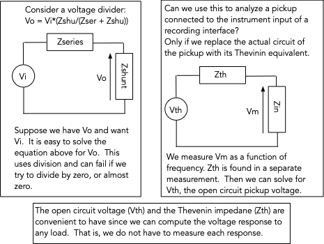
The red line is the voltage measured with an exciter coil with the pickup connected directly to the input of a recording interface with an input resistance of 1 M and a capacitance of 160 pf.  The blue line is a computed approximation of the open circuit response.  It requires as inputs the loaded measurement, the input impedance, and the pickup impedance.  Notice that the peak frequency of the computed response is slightly higher than that of the measurement in the current discussion on string based exciter coils, which was made with a preamp with a lower capacitance than the interface (but not zero, of course).

I will describe how the computation is accomplished in the next post, using Thevenin's theorem (https://en.wikipedia.org/wiki/Thévenin%27s_theorem), with the extension to ac circuits.  This theorem says that a circuit composed of an arbitrary number of impedance elements, as well as voltage and current sources, can be replaced by an equivalent circuit with a single impedance in series with a single voltage source.  The impedance is found by setting the voltages sources to zero, but leaving them in place as shorts, and removing the current sources.  The impedance between the two terminals is then found. Thus, this impedance is the pickup impedance we measure.  However, we do not have the open circuit voltage, but rather a voltage measured into a load, all be it a fairly high impedance, but not infinite.  The problem then is to find the open circuit voltage (as a function of frequency) from the load voltage and the impedance.  This is not hard, but is left for the next post.

[ms]

Some thing appears to be wrong with what I have done, and so I have removed the explanation.  I will work on it some more!  OK, I had some connection issues with my equipment, and I was puzzled that my "Christmas present" recording interface has more than twice as much input C on insdtrtument channel 1 as on 2.  (That is just the way it is since the switching on the two channels is different.  So I am putting back this explanation.







Also, here is an example of what you can do with both kinds of measurements used together:

[quadnutz]

The Hohner licensed by Steinbeger guitars have a claim blend circuit that emulates a split of the rail humbucker pickups by a resistor capacitor network:
music-electronics-forum.com/filedata/fetch?id=855597&d=1568717696

[ms]

Compare calculated and measured loaded responses.

In the figure below the red is the measured amplitude of the response, and the magenta is the measured phase.  The curves to the right of these are the computed open circuit responses.  The curves to the left show the responses when loaded with 500 pf and 500 K ohms in parallel, shown two ways. The underneath solid color curves are the computation from the open circuit response, while the dashed curves are a measurement with that load.  There is near perfect agreement.

[JohnH]

A nice clear graph, and clearly what you are doing to relate open circuit to loaded parameters has worked realy well. Can you now also plot the Thevenin impedance vs frequency? (impedance ohms and phase) and would the phase related to that impedance be the same or different to the open-circuit phase plotted above?

If its possible to output those parameters of open-circuit voltage, impedance and phase, then its a signature for that pickup that can be fed into any analysis of the circuitry downstream using classical theory.

[ms]

Feb 18, 2023 15:21:30 GMT -5 JohnH said:

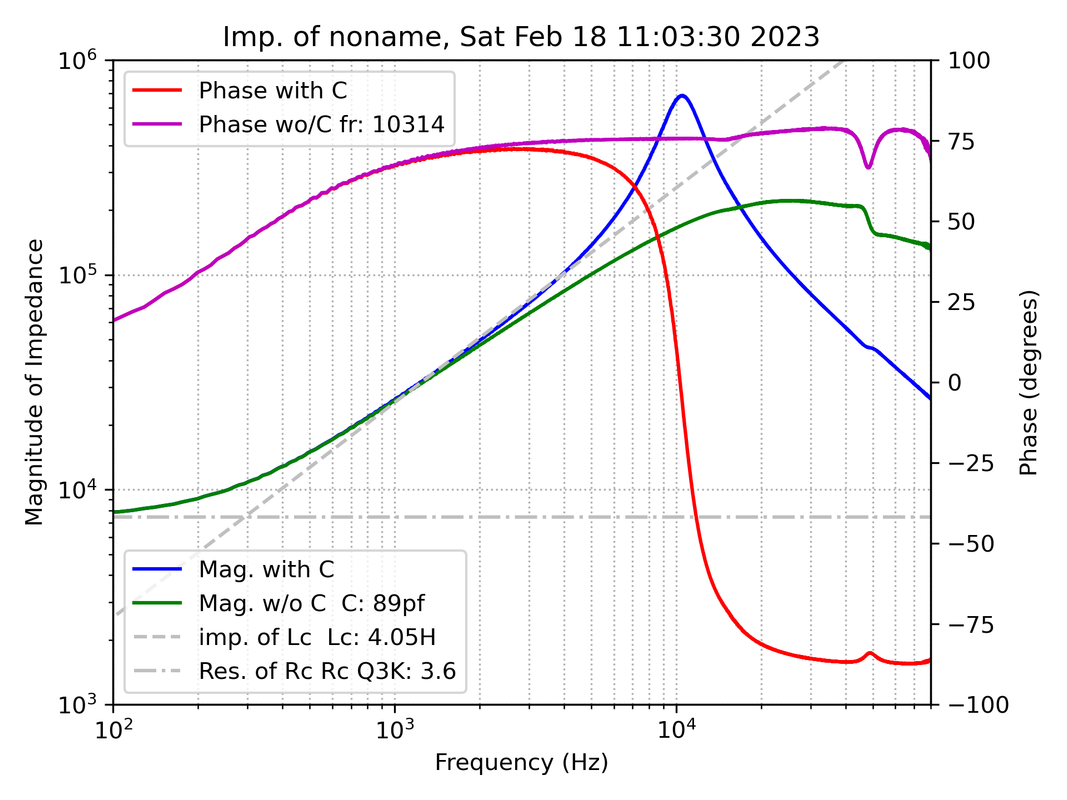
A nice clear graph, and clearly what you are doing to relate open circuit to loaded parameters has worked realy well. Can you now also plot the Thevenin impedance vs frequency? (impedance ohms and phase) and would the phase related to that impedance be the same or different to the open-circuit phase plotted above?

If its possible to output those parameters of open-circuit voltage, impedance and phase, then its a signature for that pickup that can be fed into any analysis of the circuitry downstream using classical theory.

The process of making the loaded response from the the Thevinen equivalent uses the open circuit voltage, both amplitude and phase, and Thevinen impedance, both amplitude and phase.  The plot in the first post shows both amplitude and phase of the open circuit voltage.  The plot below shows the amplitude and phase of the impedance two ways.  We need it with the effect of the C included, of course, and that is the blue and red lines. The lines with the C "unparalleled" are useful for showing that the L is more than just a simple L.  One of the advantages of using a Thevinen representation for storing the information necessary to predict the response with any load is that we do not have to explicitly deal with the complexities of the inductor; we just need the measurements.


For further processing in Matlab and related applications, it would be convenient to store and retrieve the information in an hdf5 file.  I was thinking that this would work for Excel as well, but as far as I can determine you cannot input into Excel from hdf5.  It would be necessary to agree on some ASCII format.

[aquin43]

I thought of characterising a pickup this way as well, but the problem as I see it is that you need a table driven simulator to use the results. I can't see how to make Spice, for example, do that.

That is why I followed the route of modelling the impedance with L//R sections and a capacitor. This gives you a model which is generally useful below the open circuit resonance with most pickups. I have found that it is usually the mini humbuckers that give trouble above the open circuit resonance because of fairly tight coupling between the coils.